Wool Economics 101
In our lamb analysis this week we have looked at the demand-based reasons as to why the Eastern States Trade Lamb Indicator (ESTLI) has been on the improve since the 2000’s. Given the market recess for wool, we thought a demand and supply retrospective would be of benefit too, in order to help explain one of the key drivers for surging wool prices.
The Mecardo Lamb analysis that focuses on demand curve shifts that have led to higher lamb prices can be viewed here.
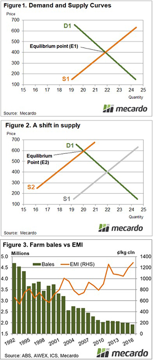
The laws of economics state that demand curves have an inverse relationship to price. This means that as prices increase the quantity demanded declines and as prices drop the quantity demanded increases. This is outlined by demand curve D1 in Figure 1.
On the other hand, supply curves have a direct relationship to price. As prices rise so does the quantity supplied and as price falls the quantity supplied is lower, as highlighted by the supply curve S1 (Figure 1).
Market forces will act to push the price to an equilibrium level where the quantity demanded is equal to the quantity supplied. This is where the demand and supply curves intersect at a price level of 400 and a quantity of 22 units – point E1 on Figure 1.
In the case of the wool market, there has been a steady decline in wool supply since the collapse of the Reserve Price Scheme in the early 1990’s and the gradual switch from wool production to cropping. As such, for every price level, the quantity of wool supplied is now lower. This can be represented on the demand and supply diagram as a shift in supply to the left, with the supply curve moving from S1 to S2 (Figure 2). The new equilibrium level (E2) under this scenario of reduced supply is shown as a price of 600 and a quantity of 20 units. In this circumstance, the price has been driven higher by a contraction in supply over time.
Analysis of the wool market supply (bales produced per year) and price (Eastern Market Indicator – EMI) since the early 1990’s confirms the theory that reduced supply has been a key driver of higher wool prices. As identified in Figure 3, annual total wool bale production has declined from over 4.5 million bales in 1992 to under 2 million bales in 2016, with the EMI more than doubling over that time frame from 600¢/kg clean to over 1200¢/kg.
Key points:
- Supply of wool has been in decline since the early 1990s and is a key underlying reason as to why wool prices have been increasing over time.
- The annual level of wool bales produced has more than halved over the last two decades which has coincided with wool prices more than doubling in value.
- In recent years the wool supply has stabilised, yet prices have continued to climb suggesting demand led factors are behind the current market rally.

